
From QGIS labels to a new-construction detector and a new dataset in an hour
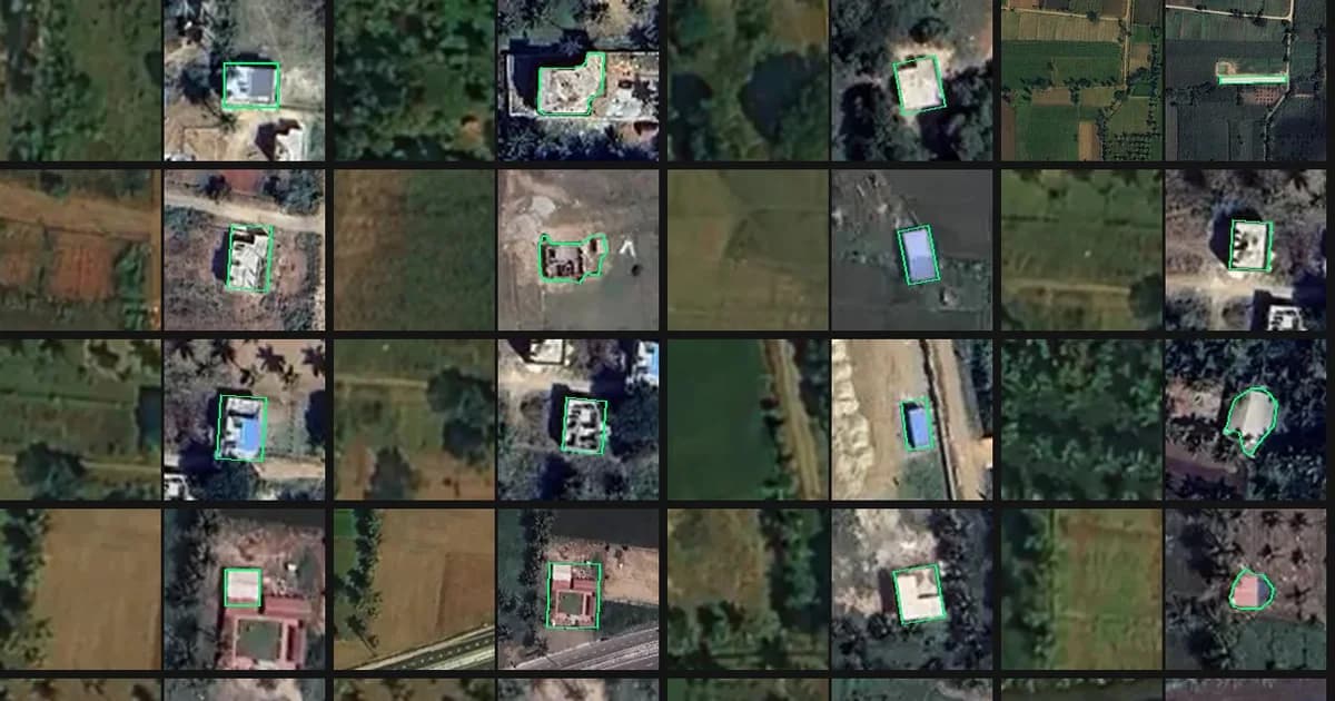
We keep experimenting with AI Agents and now it's the case of mapping validation and construction detection. It's worth saying this is yet another disruptive workflow in AI mapping. In this particular experiment we gave an AI agent a QGIS project having 487 hand-drawn polygons, and asked: are these labels good enough to train a detector for low-rise new construction? About 30 minutes later it had trained a change classifier on them and checked every label. It flagged 10% of the labels to remove or fix and found new buildings our cartographers have missed.
The task
Preliminary project
Our project area was in Karnataka, India, about 9 × 8 km. It mixes dense town blocks with villages, palm plantations and farmland. The target is new low-rise construction: mostly one- and two-storey houses, sheds, and freshly cleared plots.
- The initial dataset was created with the Mapflow plugin for QGIS. Construction sites were manually labeled as bbox or convex hull areas and then the Mapflow Buildings model was applied to outline the buildings within these areas.
- Based on the annotation results we estimated the possible accuracy of the model for construction detection as ~70% for 90% of construction sites.
- Classification of construction by the stages was expected to be lower with a wider confidence interval. To increase this accuracy, we required customers to use more detailed imagery like aerial photographs, which appeared to be costly and didn't fit the project's budget, so we abandoned this idea.
The Agentic workflow
The input for Agent was:
- A QGIS project (.qgz) with two imagery layers: a global mosaic from 2023 ("before") and a new high-resolution scene ("after").
- A GeoJSON of 487 construction-change polygons with a
stageattribute (completed / new / empty). Only 110 labels had a stage, too few to learn from, so the classifier was tasked to ignore it and treat every polygon as one "construction change" class.
The prompt was one sentence: use these labels as training labels for construction changes, validate them, and find missing or false labels.
What the agent did
The agent read the project, defined the steps, and wrote and ran its own scripts.
- Read the QGIS project
- Pulled the imagery
- Aligned the dates. Here is the interesting point! The images were 3–8 m apart, and the offset varied across the scene. The agent measured the shift on a grid of image windows and warped the 2023 mosaic onto the new one, which brought the remaining error down to about 0.8 m.
- Looked at every label. It cut a before/after chip for each of the 487 polygons and reviewed them in sheets of 28. It then reopened about 90 doubtful ones at larger size.
- Trained a classifier on the labels. It ran a pretrained ResNet-18 over both dates and trained a logistic regression on the two dates' features and their difference. It tested on spatial blocks the model had not seen: AUC 0.96.
- Hunted for misses. It ranked unlabelled places by "looks built now, looked unbuilt in 2023". It reviewed the top 108 candidates one by one and sampled further down the list to estimate how many were missed.
- Handed back the results. It produced a GeoJSON of the labels with a
qa_flagper polygon, a list of candidate misses, and a report page with the image chips.
What it found
Of the 487 labels, 88% were correct, and the problems clustered into a few patterns.
| Issue | Labels | What it looks like |
|---|---|---|
| Already built in 2023 | 23 | The house is in both images, or nothing changed at all |
| Roof change only | 14 | Same footprint; a green roof became blue, or a red one orange |
| Over-drawn polygon | 9 | The box covers an old house plus its new extension; one is 2.4 ha |
| Demolition | 3 | Sheds removed, nothing built |
| Uncertain | 8 | Roof on existing walls, or just a re-roof? The 2023 image is too soft to tell |
The bigger finding was what was missing. In the top 108 ranked candidates the agent confirmed 39 unlabelled new buildings and 29 construction sites or cleared plots. Samples further down the list added a few more. Extrapolating the hit rates, the scene likely holds 100–200 unlabelled new buildings, so building recall is roughly 70–80%. Note this is how complete the hand labels are, not the model's accuracy, so it doesn't yet check our preliminary ~70% estimate.
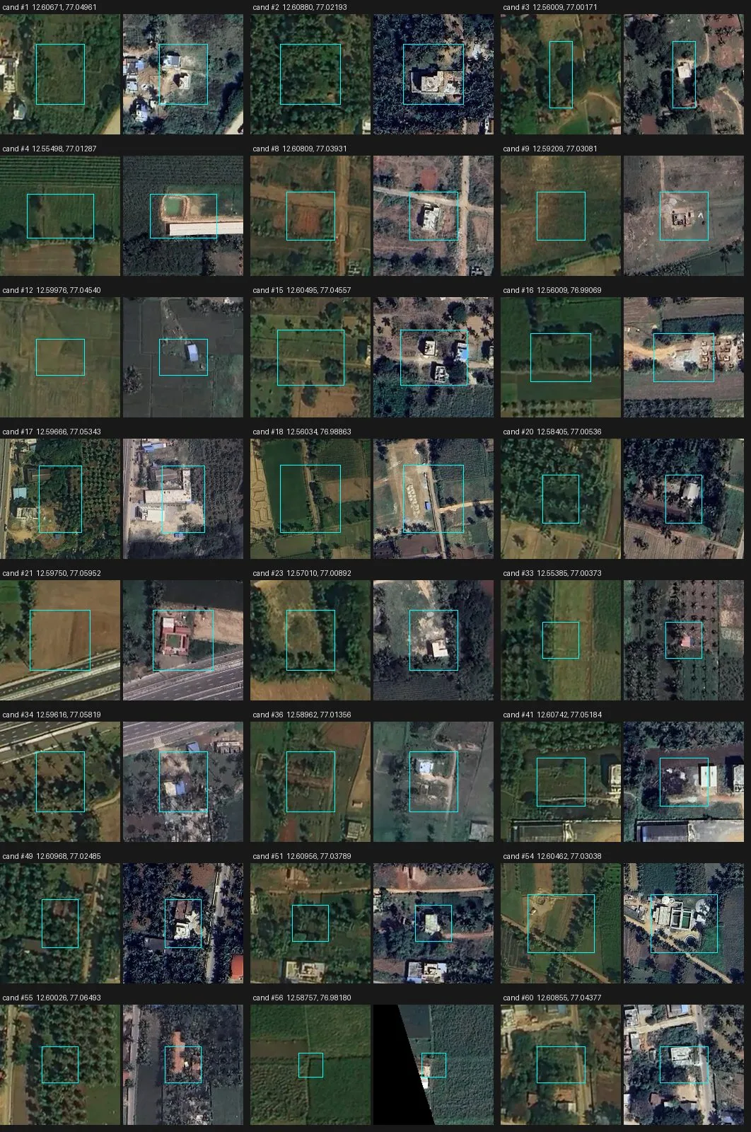
Missed new buildings found by the classifier. The cyan box marks the candidate: empty land in 2023 (left), a new house or shed now (right).
Rural and dense urban fail differently
The two settings break labels in opposite ways, so a training set needs both covered on purpose.
- Rural areas: misses. Most unlabelled buildings were lone houses in palm groves, sheds by fields and new compounds on village edges. Of the 42 confirmed misses, 35 had fewer than five labels within 500 m, and most had none. Annotators concentrate where change is dense and skip the empty-looking tiles - this is how our annotation workflow was built in QGIS (toggle old <> new imagery layers and catch the difference by eye). A model trained on that learns to ignore isolated construction.
- Dense urban areas: false labels. About 9 in 10 false and roof-only labels sat in dense clusters, with five or more other labels within 500 m. When roofs are packed together, a blue re-roof or a new storey looks like a new building (also a human eye factor), and a soft 2023 image makes it worse.
- Annotators need a written policy for edge cases. Re-roofs, extensions, demolition and bare land clearing were each labelled in some places and not in others.
- Align the images before cutting chips. A few metres of offset turns every unchanged house edge into a fake "change" pixel. This matters most in dense areas, where buildings are small and touch each other.
Closing the loop with Mapflow
The agent then added 45 missing buildings to the training set itself. It took about 12 minutes in a Mapflow SAM session, connected through MCP.
- The agent placed one point on each missed building at the 42 confirmed locations. Mapflow's magic wand outlined each building from its point.
- Its first try used a coarse 2.3 m scale and drew loose shapes. Switching the wand to 0.29 m fixed them. The agent adjusted this parameter itself.
- A contact sheet of every outline caught four misses: a compound wall, paving, a dark patch and bare ground. The agent deleted them and squared the rest into rectangles.
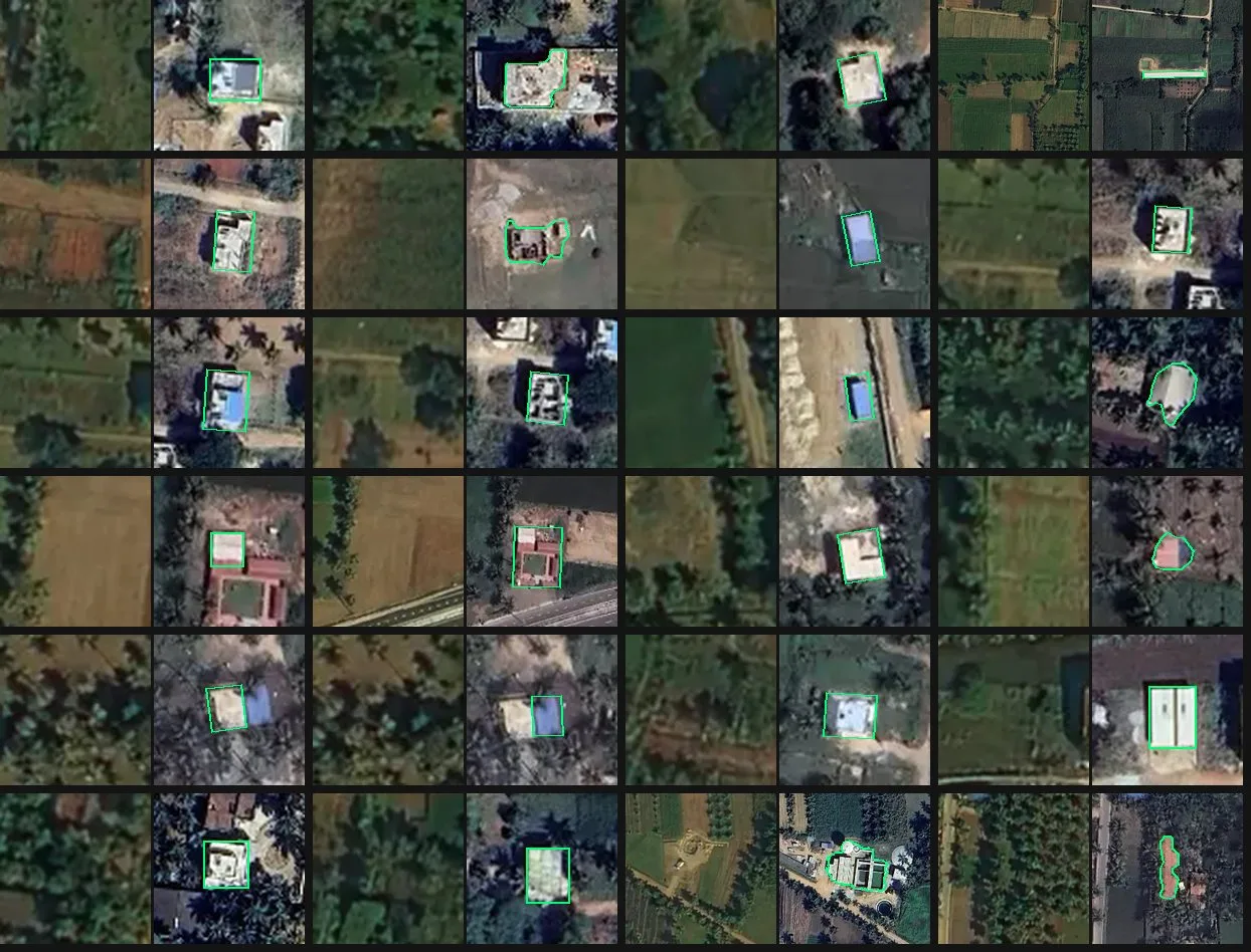
24 of the 45 new footprints. Each pair shows the 2023 image on the left and the new image with the Mapflow outline on the right.
The result merges straight into the training labels: the 446 labels kept after QA plus 45 new footprints, 491 in all.
Effort, cost and next steps
The agent run took about 26 minutes and about $6.30 in model usage. Reviewing 487 before/after pairs and scanning 75 km² for misses by hand would take our annotators a couple of days or more.
The whole session of QA mapping came to about $31. The table shows the breakdown by step, from the session's usage log. The model is Claude Opus 5.5, one of the most expensive.
| Step | Agent steps | Price-weighted tokens | Cost (USD) |
|---|---|---|---|
| Label QA: tiles, alignment, classifier, review, report | 73 | 2.28M | 6.31 |
| Mapflow SAM footprints (total) | 61 | 2.75M | 7.59 |
| Upload image to Mapflow, prepare session | 15 | 0.51M | 1.40 |
| Pick seed points on 42 locations | 19 | 1.12M | 3.10 |
| SAM session: wand, review, rectangles, export | 17 | 0.68M | 1.89 |
| Update post and project doc | 10 | 0.43M | 1.19 |
| Blog post draft | 13 | 0.73M | 2.01 |
| Edits from comments | 55 | 4.44M | 12.28 |
| Project doc fix | 5 | 0.61M | 1.67 |
| Usage check | 8 | 0.30M | 0.82 |
| Total | 215 | 11.1M | ~31 |
The table counts only the agent's model usage. The Mapflow area fee comes on top. At $1 per km² with a 1 km² minimum, it would be about $75 for the whole scene. Sending only 200 m windows around the 42 missed buildings, as one multi-part area, brings it to about $2. Outlining all new buildings needs about 5% of the area, $4 (see the scaling table).
Could the agent have outlined the 45 buildings without SAM? It would still need the seed points ($3.10), then draw each polygon by eye and check and fix them over 2–3 rounds, about 25 more steps. That comes to about $6 in tokens, about the same as the SAM route ($5 in tokens plus a $2–4 Mapflow fee). The difference is in quality. Hand-placed corners on 0.58 m imagery are off by 1–2 pixels, about 1 m, which is roughly a 25% area error on a 150 m² house. SAM snaps outlines to roof edges.
Scaling to all of Karnataka
At state scale the cost moves almost entirely to the Mapflow area fee. Agent tokens become a small fixed cost, and that depends on three optimisations:
- Change detection runs as code. The trained classifier runs as plain code with no agent in the loop. The features took about 340 CPU-seconds for this 75 km² scene, about 4.5 s per km².
- The agent only reviews. It checks a sample of about 200 detections per district rather than every label.
- SAM only sees change windows. Outlining runs on 100 m windows around detections, sent as one multi-part area per district. No per-building wand clicks.
In Maddur, 100 m windows cover 5% of the area for the true new buildings and 16% for everything the current detector flags. The table assumes 5% of the area goes to Mapflow: 100 m windows around all new buildings, each district sent as one multi-part area. The 42 missed buildings alone needed 2%.
| Scale | Area (km²) | Area sent to Mapflow (5%) | Detection compute | Mapflow fee at $1/km² | Agent tokens | Total | Per km² |
|---|---|---|---|---|---|---|---|
| This test (Maddur) | 75 | 3.8 km² (billed as 4) | < $0.01 | $4 | $11 | $15 | $0.20 |
| One district (avg) | 6,200 | 310 km² | ~$1 | $310 | ~$10 | ~$321 | $0.052 |
| Karnataka (31 districts) | 191,800 | 9,590 km² | $30–50 | $9,590 | ~$350 | ~$9,980 | $0.052 |
| For comparison: whole state sent to Mapflow | 191,800 | 191,800 km² | $30–50 | $191,800 | ~$350 | ~$192,200 | $1.00 |
Agent tokens at state scale come to about $20 for building and retraining the pipeline, plus about $10 per district for sample review and running Mapflow. Running the full agent QA scene by scene instead would cost about $16,000 (2,560 scenes × $6.30). Imagery is not included. Neither is the cost of retraining to raise detector precision, which shrinks the windows and the fee.
Conclusions
These are less closing points than a snapshot of our current experiments with a fast-shifting technology.
The Agentic based workflow leveraging scalable GPUs with an open model (Mapflow case) is a powerful method for time-consuming validation mapping tasks: more accurate and faster than the agent solo workflow, at about the same cost. At state scale the optimised workflow is about 1.6× cheaper than running the agent scene by scene ($10k vs $16k) and about 20× cheaper than running Mapflow over the whole Karnataka. Wow that's a huge difference.
It doesn't exclude the cartographer; it puts them in different shoes: annotator + supervisor. Next, we retrain on the cleaned, co-registered pairs and run the same audit again to measure the gain on the new territories.
Writing this post took us longer than training a classifier and running the agentic pipeline (not counting the initial imagery annotation).
We are in a time of transformative change, no surprise. What still surprises us is how fast it moves.
Happy Mapping! 🗺️